Gerrymandering - Study Fairness of Political Redistricting using MCMC
What is gerrymandering?
Consider a two-party state X where 30% of voters vote for blue and 70% of voters vote for red. You’d expect that X’s elected representatives would therefore be 30% blue and 70% red. But this is not the case in X. Instead, 60% of X’s representatives are blue, and 40% are red.
This is because in 2010, blue gerrymandered X. That is to say, blue redrew X’s electoral district boundaries to their advantage - they minimised the amount of “wasted” votes for their own party and maximised the amount of wasted votes for their opponents. We consider votes for blue to be wasted in districts where blue lost, because these votes could instead have been used to tip a closer election in blue’s favour in a neighbouring swing district. Similarly, in a district where blue won, a significant surplus in votes for blue are also wasted votes – a district only gets one representative for state X, which will be from the winning party regardless of whether this party received 80% of the votes or 55% of the votes in this district. These surplus votes would have been better spent elsewhere.
To illustrate this, consider the pictures below.
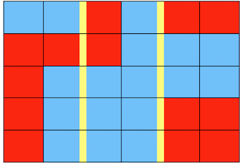
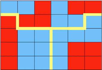
Each square block represents an equal number of voters, who all vote for the party of their colour. The rectangle represents the state that these voters live in. Suppose that the state must be divided into 3 districts with equal population, where each district holds a winner-take-all election to establish a representative. A straightforward drawing of state lines, as illustrated in the first figure, results in 1 red district, 1 blue district, and 1 tie. However, blue has more votes than it needs in the middle district. In the second figure the district boundaries have been manipulated for the advantage of the blue party, in such a way that the number of “wasted” votes for blue has been minimised. Thus we can obtain 2 blue districts and 1 tie, with the exact same votes.
So now that we understand how gerrymandering works, how can we detect if a state has been gerrymandered? A commonly thought characteristic for gerrymandering is weirdly-shaped district boundaries (hence the name gerrymandering - originating from a shape resembling a salamander and the name of the person (Governor Elbridge Gerry) who first introduced the term [1]). Therefore, compactness of the drawn districts has often been used as a measure of fairness. However, this is neither a necessary nor sufficient condition for detecting gerrymandering [2]. Sampling methods offer a viable alternative.
Using MCMC to study gerrymandering
One can use Markov Chain Monte Carlo (MCMC) to generate a range of potential district maps. Moves consist of swaps between neighbouring blocks of voters in different districts and are accepted/rejected with a Metropolis-Hastings step. One can define an energy function using ideas from statistical physics [3], where low-energy states will correspond to “better” district maps, because these low-energy maps will better fit a set of pre-determined characteristics (such as compactness of the map) which we want good maps to obey. Low-energy states, i.e., “good maps”, are visited more frequently by the sampling algorithm.
Now a district map can be set up in a statistical physics framework - using a few steps:
- Consider each block of voters to be a node in a graph structure.
- Draw connections between neighbouring nodes, even if these neighbours are located in different districts.
- Associate each node with the district it belongs to. For a two-district system we do this using an Ising spin model, where each node has a spin associated with it which either points up or down, depending on which district belongs to. Neighbouring nodes which have the same spin will have an interaction energy. For a multiple-district system one can use the generalized version of the Ising model, which is called the Potts model. Each district has a different 'spin' or color associated with it, and nodes assume the color/spin of the district they belong to.
- Define an energy function for the map, which consists of different terms that measure how well the district map obeys certain desirable criteria. Examples of such criteria would be compactness of each district and that the population of each district is about the same size. Lower energy maps better obey these criteria and are therefore desirable.
A MCMC algorithm will then work as follows:
- Running the MCMC algorithm will change the color/spin of nodes, which will affect the energy of the newly created district map.
- We accept a proposed MCMC move, i.e., a move of a node to a neighbouring district, with a Metropolis-Hastings step. If the move resulted in a map with a lower energy than the previous map, the move is more likely to be accepted. It is however important to also sometimes allow increases in energy to prevent the algorithm from getting stuck in local minima.
Acknowledgements:
This idea is based on work by Jonathan Mattingly at Duke University.
Together with my supervisor, Benedict Leimkuhler, I co-supervised a group of three excellent final year BSc students at the University of Edinburgh in 2019-2020, who used MCMC techniques to study gerrymandering in the UK.
References
[1] E. Griffith. The Rise and Development of the Gerrymander. Chicago: Scott, Foresman and Co, 1907.
[2] H. Young. Measuring the Compactness of Legislative Districts. Legislative Studies Quarterly, 13(1):105-115, 1988.
[3] C. Chou and S. Li. Taming the Gerrymander—Statistical physics approach to Political Districting Problem. Physica A: Statistical Mechanics and its Applications, 369(2):799-808, 2006.